Tutorial: Welcome¶

Overview¶

In this tutorial, we walk through how to build a logistic regressor in Tflon using Wisconsin Diagnostic Breast Cancer dataset as our example. We will build on this example extensively to demonstrate how to fully utilize the Tflon deep learning package and extend it with custom features. We will assume a working knowledge of pandas and object oriented programming in python. Futher, we recommend Deep Learning by Benjio as this tutorial doesn’t serve as a replacement for solid practical and theoretical understanding of deep learning.

Setup¶

Clone the latest tflon repository and ensure the following requirements:

pandas 0.21.0+
tensorflow 1.6.0+
horovod 0.13.4+
mpi4py 3.0.0+
mpirun 2.1.0+

Instalation¶

You can find the source code at https://bitbucket.org/mkmatlock/tflon, and install it using Mercurial:

hg install https://<your username>@bitbucket.org/mkmatlock/tflon/src/default/
pip install ./tflon

Imports¶

Before using tflon in python, we use the following lines to import the necessary dependancies

import pandas as pd
import tensorflow as tf
import tflon

Environment Reset¶

By the nature of Tensorflow which maintains a stateful representation of the network being trained. In order to instantiate another network, we have to reset the system with

tflon.system.reset()

This will reset the tensorflow stored network. So, that you can define and train another model within the same python file or jupyter notebook kernel.

Example Dataset¶

For the purposes of this tutorial, we will be using the Wisconsin Diagnostic Breast Cancer (WDBC) dataset found at https://archive.ics.uci.edu/ml/machine-learning-databases/breast-cancer-wisconsin/wdbc.data

The data has 30 real valued features including

radius (mean of distances from center to points on the perimeter)
texture (standard deviation of gray-scale values)
perimeter
area
smoothness (local variation in radius lengths)
compactness (perimeter^2 / area - 1.0)
concavity (severity of concave portions of the contour)
concave points (number of concave portions of the contour)
symmetry
fractal dimension (“coastline approximation” - 1)

We seek to construct a classifier to determine if the biometrics correspond to a malignant (212) or benign (357) using the 569 samples.

Logistic Regressor¶

Check out http://www.win-vector.com/blog/2011/09/the-simpler-derivation-of-logistic-regression/ if you’re not familiar with it. Basically, you can think of it as a best linear fit of the log odds ratio minimizing the pseudo-\(R^2 = 1-\frac {\text{deviance}}{\text{null deviance}}\).

From the provided link:

Logistic regression models are multiplicative in their inputs.
The exponent of each coefficient tells you how a unit change in that input variable affects the odds ratio of the response being true.
Logistic regression is coordinate-free: translations, rotations, and rescaling of the input variables will not affect the resulting probabilities.
Logistic regression preserves the marginal probabilities of the training data.
Overly large coefficient magnitudes, overly large error bars on the coefficient estimates, and the wrong sign on a coefficient could be indications of correlated inputs.
Coefficients that tend to infinity could be a sign that an input is perfectly correlated with a subset of your responses. Or put another way, it could be a sign that this input is only really useful on a subset of your data, so perhaps it is time to segment the data.
Pseudo-\(R^2\) is a useful goodness-of-fit heuristic.

Pre-Proccessing¶

The data is in the form of comma separated values(csv): ID, Malignant/Benign, Features. Using pandas, we extract the targets (‘targ’) with a binary encoding 1 for malignant and 0 otherwise. Informally, the targets are the observed labels we are trying to learn and ‘desc’ for the descriptors which are the features we are learning from.

df = pd.read_csv("./wdbc.data" , header=None)
df[1] = df[1].apply(lambda x : 1 if (x == 'M') else 0)
df = df.iloc[:,1:]
targ, desc = tflon.data.Table(df).split([1])

Then, we create a tflon Tablefeed which essentially stores the ‘targ’ and ‘desc’ as a dictionary making for efficient training.

feed = tflon.data.TableFeed({'desc':desc, 'targ':targ})

Defining a Model¶

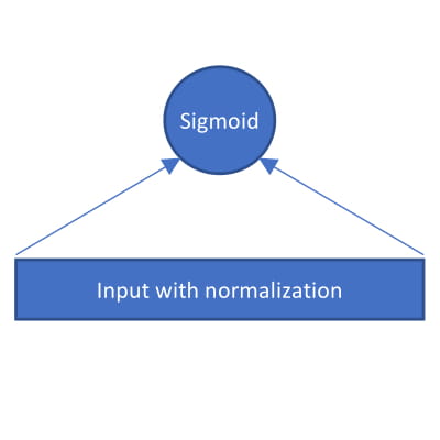
For this example, we are simply building a ridge logistic regressor so it suffices to feed the normalized input into a single dense neuron with a sigmoidal activation.

To define a new model, we define a new subclass of tflon.model.Model and override the _model attribute. Using add_input and add_target, we indicate that the input should have 30 features and a single target. Again, a target is the observed labels that we want our network to learn from.

class MyModel(tflon.model.Model):
    def _model(self):
        I = self.add_input('desc', shape=[None, 30])
        T = self.add_target('targ', shape=[None, 1])

Architecture¶

Now in defining the actual architecture, we appeal to the toolkit subpackage which has layers available for us.

WIn = tflon.toolkit.WindowInput()
Dense = tflon.toolkit.Dense(1)
net = WIn(Dense)
out = net(I)

To be more concise, we can stack layers ontop of each other with the ‘|’ symbol allowing us to construct L which is the instantitation of the defined architecture

net = tflon.toolkit.WindowInput() |\
      tflon.toolkit.Dense(1)

out = net(I)

In the case of the WindowInput function, it normalizes each feature with the following function

\[\frac {x - min}{max-min}\]

As for Dense(\(x\)), it simply constructs fully connected neuron layer with \(x\) neurons. For us, we only use 1 neuron, so \(x = 1\).

To be truly minimalistic, this layer can be skipped all together:

net= tflon.toolkit.Dense(1)

This is the main area of design for customizing the model that we build. Additionally, the recommend way of adding new custom functionality to tflon is by adding a new layer with the ‘|’ symbol. We’ll discuss in more detail how to define new layers here

Prediction¶

The prediction is the final pass made on the output which in our case by choosing sigmoidal activation we result in a logistic regressor.

self.add_output( 'pred', tf.nn.sigmoid(out) )

Objective Function¶

In a logistic regressor there is a objective function or a cost function that is minimiazed to definine the best fit. The L2 is an artifact of our choice to build a ridge regressor.

self.add_loss( 'xent', tflon.toolkit.xent_uniform_sum(T, out) )
self.add_loss( 'l2', tflon.toolkit.l2_penalty(self.weights) )

Checkout the full list of loss functions in the toolkit here.

Metrics¶

Finally, we define some metrics that allow us to judge the performance of our logistic regressor. In particular, here we have used the Area Under the Reciever Operating Characteristic curve (AUC) as our metric which gauges sensitivity (true positive rate) and specificity (false positive rate). We can then retrieve the value later as will be mentioned shortly.

self.add_metric( 'auc', tflon.toolkit.auc(T, out) )

Putting it together¶

``` python class MyModel(tflon.model.Model): def _model(self): I = self.add_input(‘desc’, shape=[None, 30]) T = self.add_target(‘targ’, shape=[None, 1])

net = tflon.toolkit.WindowInput() |\
      tflon.toolkit.Dense(1)
out = net(I)

self.add_output( 'pred', tf.nn.sigmoid(out) )
self.add_loss( 'xent', tflon.toolkit.xent_uniform_sum(T, out) )
self.add_loss( 'l2', tflon.toolkit.l2_penalty(self.weights) )
self.add_metric( 'auc', tflon.toolkit.auc(T, out) )
```

Train the Model¶

To train the model, we first instantiate the model and define our trainer:

python LR = MyModel() trainer = tflon.train.OpenOptTrainer( iterations=100)

Then exactly synonomous to tensorflow, we execute the training from within a session which can be thought of as denoting an environment after which background bookkeeping will be erased.

with tf.Session():
    LR.fit( feed, trainer, restarts=2 )
    metrics = LR.evaluate(feed)
    print "AUC:", metrics['auc']

Note that here we are able to use evaluate to retrieve our AUC.asdf

Save and Load Trained Model¶

Once we’re trained a model we want to be able to reuse it in the future. So it’s crucial that we mention how to save and load models here.

To save a model we simply use the save function within the session but after we do the fit. This will produce a pickle file

LR.save("saved_lr.pkl")

Then next time when we want to load the model back, we can simply use load. Note that you have to manually initialize the model before use.

LR = tflon.model.Model.load("saved_lr.pkl")
with tf.Session():
    LR.initialize()
    x = LR.evaluate(feed)
    print "AUC:", metrics['auc']

Putting it all together¶

Congratulations our ridge logistic regressor is ready!

import pandas as pd
import tensorflow as tf
import tflon

class MyModel(tflon.model.Model):
    def _model(self):
        I = self.add_input('desc', shape=[None, 30])
        T = self.add_target('targ', shape=[None, 1])

        net = tflon.toolkit.WindowInput() |\
              tflon.toolkit.Dense(1)
        out = net(I)

        self.add_output( 'pred', tf.nn.sigmoid(out) )
        self.add_loss( 'xent', tflon.toolkit.xent_uniform_sum(T, out) )
        self.add_loss( 'l2', tflon.toolkit.l2_penalty(self.weights) )
        self.add_metric( 'auc', tflon.toolkit.auc(T, out) )

if __name__=='__main__':

    df = pd.read_csv("./wdbc.data" , header=None)
    df[1] = df[1].apply(lambda x : 1 if (x == 'M') else 0)
    df = df.iloc[:,1:]
    targ, desc = tflon.data.Table(df).split([1])
    feed = tflon.data.TableFeed({'desc':desc, 'targ':targ})

    LR = MyModel()

    trainer = tflon.train.OpenOptTrainer( iterations=100)

    with tf.Session():
        LR.fit( feed, trainer, restarts=2 )
        LR.save("saved_lr.p")
        metrics = LR.evaluate(feed)
        print "AUC:", metrics['auc']

Sample Output¶

2018-06-11 13:28:38.304284: I Found a solution with loss 7.27e+01 AUC: 0.99299717